
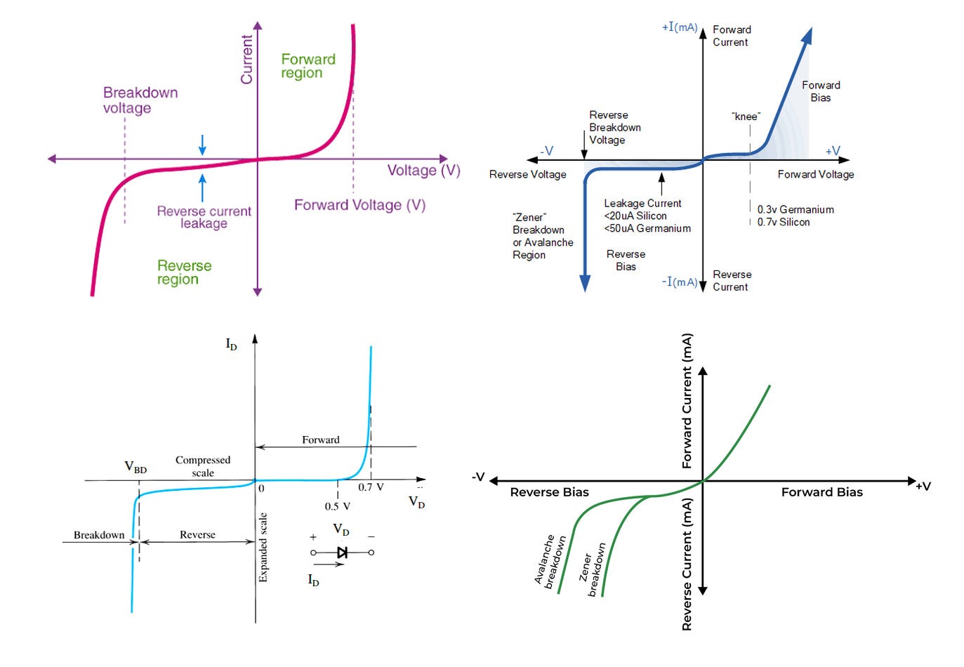
When working on my latest book, The Secret Life of Circuits, I wanted to keep the artwork real. My beef with the diagrams in popular electronics textbooks and online tutorials is that most of them are fake. At best, they’re retraced from ancient texts; at worst, they’re sketched from memory and can be charitably described as “inspired by true events”:
The Secret Life of Circuits contains about 290 original illustrations and does its best to avoid such shenanigans. I painstakingly gathered real data for everything from quartz crystal frequency response, to battery discharge curves, to signal reflections in a 100 ft run of coax cable strewn around the workshop, to the behavior of vacuum tubes.
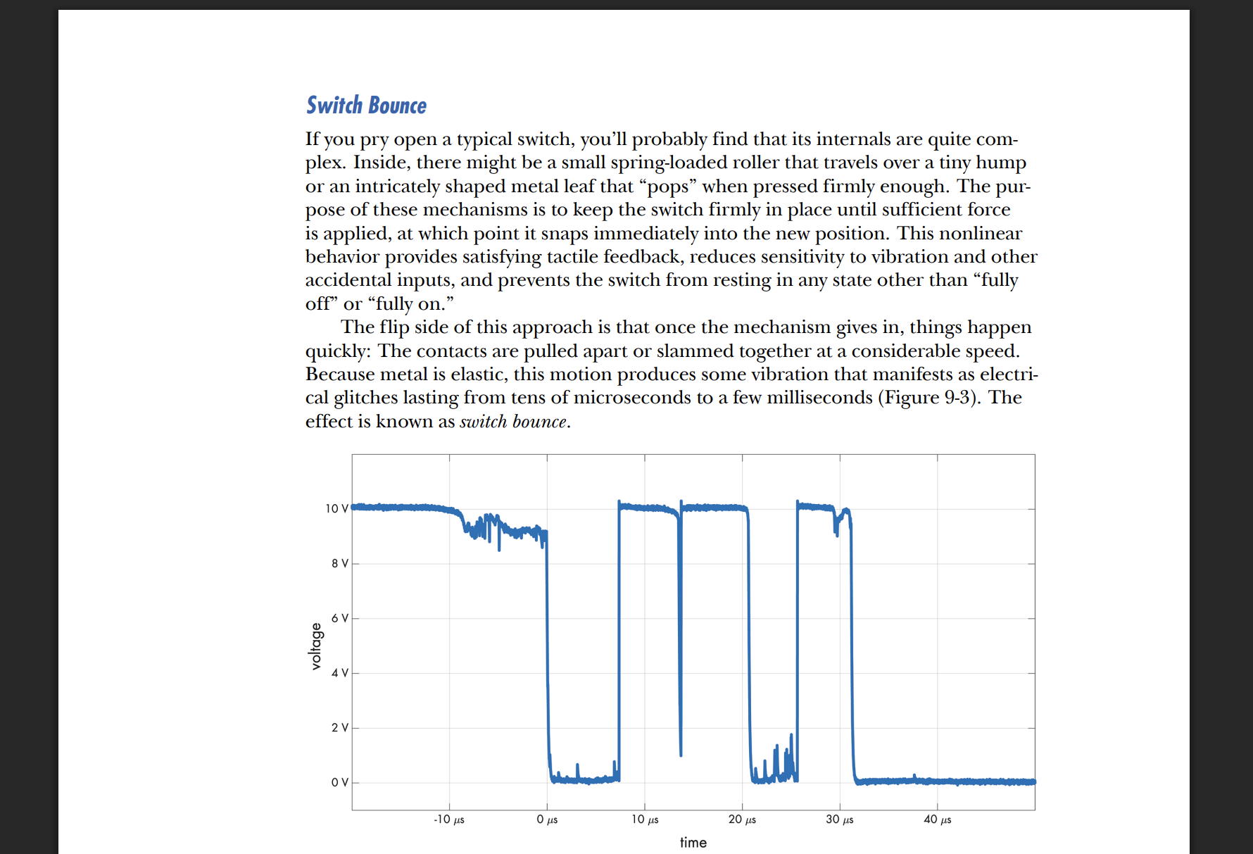
Most of it was straightforward to capture, but I can’t say the same about the parametric plots that show the relation between voltage and current in semiconductor devices. In some portions of the curve, the currents are too miniscule to record with the most common graphing instrument, the oscilloscope. In other portions, the current suddenly skyrockets — and before you know it, the device lets out the magic smoke. Even in the in-between region, there’s no respite: the characteristics of semiconductor junctions change with temperature, and that includes self-heating due to currents as low as 1 mA. Do nothing and watch a point on the oscilloscope screen drift away.
To tackle this problem, I ditched the oscilloscope in favor of a benchtop multimeter (DMM) and pulsed power from a lab supply. The perk of the multimeter is that it can easily measure down to microamps and microvolts; the perk of pulsed power is that heating-indued drift can be kept in check.
Oh — I would also submerge the device under test in non-conductive liquid for cooling purposes. Mineral oil is a sensible choice, but many other options should do:
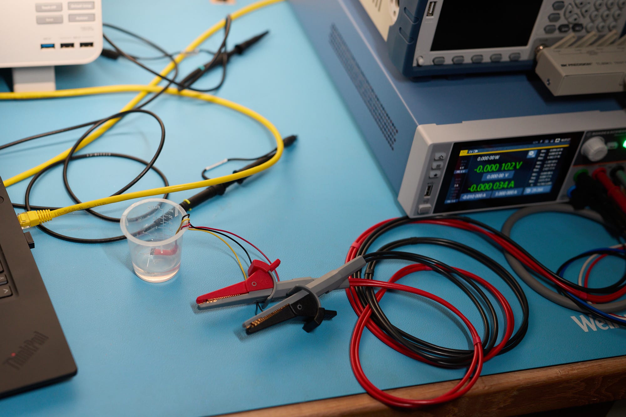
Although I prepared some diagrams by manually writing down currents and voltages, this is obviously tedious and error-prone, so it’s better if one or more of the instruments can be interfaced to a computer. Many benchtop instruments support a simple, text-based protocol called Standard Commands for Programmable Instruments (SCPI). Depending on the age of your gear, the interface may be available over RS-232, via a USB Type B (printer-style) port on the rear, or via Ethernet — in which case, you simply establish a TCP connection to port 5025.
The SCPI protocol uses commands and queries. An example of a query is *IDN? followed by a newline (\n); sending this string causes the device to respond with a line of text describing its make, model, and other identifying information. Another possible query is MEAS:VOLT?, which might return the current voltage reading. In contrast to queries, commands do not return any text; an example may be SOUR:VOLT 1.2 to set the voltage to 1.2 V, or OUTP 1 to turn on output channel 1.
Alas, although I had an SCPI-capable multimeter, my benchtop power supply was more basic and offered no remote control; without it, the process was still half-manual. Fed up, I eventually purchased a source measure unit (SMU) — essentially a combination power supply and a multimeter with a very fast response time. Brand new SMUs are obscenely expensive, but there are virtually no second-hand buyers for them, so it’s easy to find excellent deals on eBay if you haggle a bit. I scored an unmolested Rohde & Schwarz NGU401 unit for a laughably tiny fraction of its astronomical MSRP ($9,000).
This particular SMU can be used by repeatedly setting the output voltage and then querying the DMM for the current on-screen reading, but the reading is updated only at a frequency of about 3 Hz. A better option is to use the device’s data streaming mode; in the Rohde & Schwarz parlance, this is known as FastLog. The API allows sampling rates of 100 to 500k per second (!) and sends voltage-current pairs as binary 4-byte floats.
Of course, as can be expected of a niche feature on a niche device, nothing actually works as documented. The most grievous problem is that the returned binary data is corrupted if you try to use the serial-over-USB interface; after a day of chasing ghosts, I was finally able to get it to work over Ethernet.
My C implementation for capturing the V-I curve of a forward-biased diode can be found here. It uses FastLog at 10 ksps; for currents below 0.3 mA or so, it leaves the supply voltage on and averages 2,500 data points to obtain a noise-free microamp-range reading. For higher currents, it cycles the power on for 5 ms and averages the best 20 samples from the FastLog buffer.
The following plot shows the actual, positive-side V-I curve for a popular, small 1N4148 diode with a continuous current rating of 300 mA:
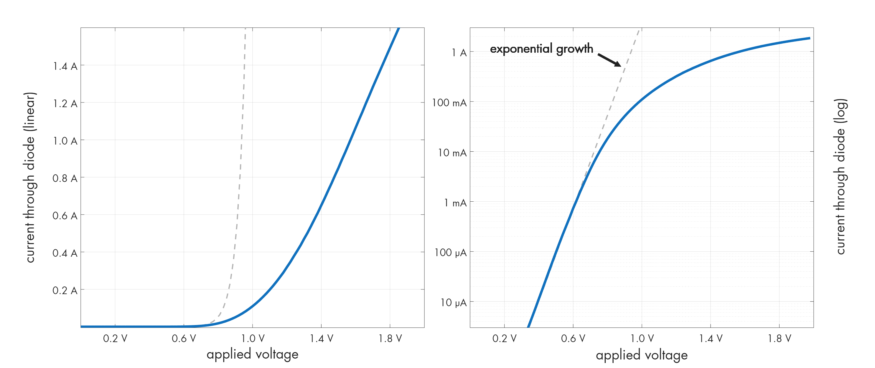
Unedited measurement data can be found here. I was able to effortlessly cover the range from few microamps to nearly 2 A; it’s actually possible to go to 4 A, but it adds no interesting detail to the plot.
Note that although the relation between the applied voltage and current in a diode is often described as exponential, this is true only for modest currents. In the log-current plot on the right, we see that the property no longer holds in the vicinity of 10 mA; the curve diverges from the dashed line that represents an idealized model fitted to the initial, truly exponential slope. That’s because of resistive effects in the semiconductor substrate — and it’s one of many reasons why it pays to have real plots.
Diodes eventually begin to conduct when reverse-biased too, but in the case of 1N4148, the threshold is about -145 V, so it’s hard to capture all of the component’s dynamics on a single well-proportioned plot. We can do it more easily for Zener diodes. For example, the following was captured for 1N4731, a relatively beefy, low-voltage Zener rated for 4.3 V at 58 mA:
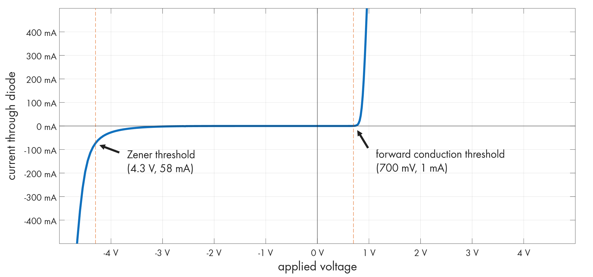
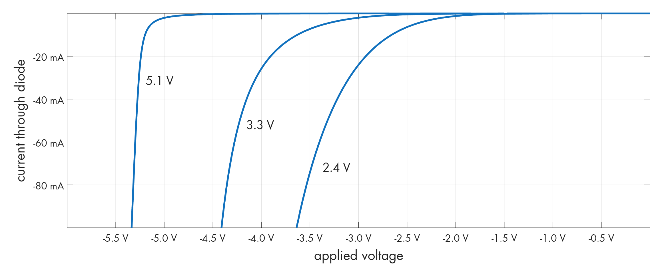
In low-voltage Zener diodes, reverse breakdown curve is not as steep as the response in forward bias; if you want the component to produce the specified reference voltage, the current flowing through needs to be matched reasonably well. Taking measurements for another type of Zener diodes (BZX79), we can see that the knee gets sharper past circa 5 V:
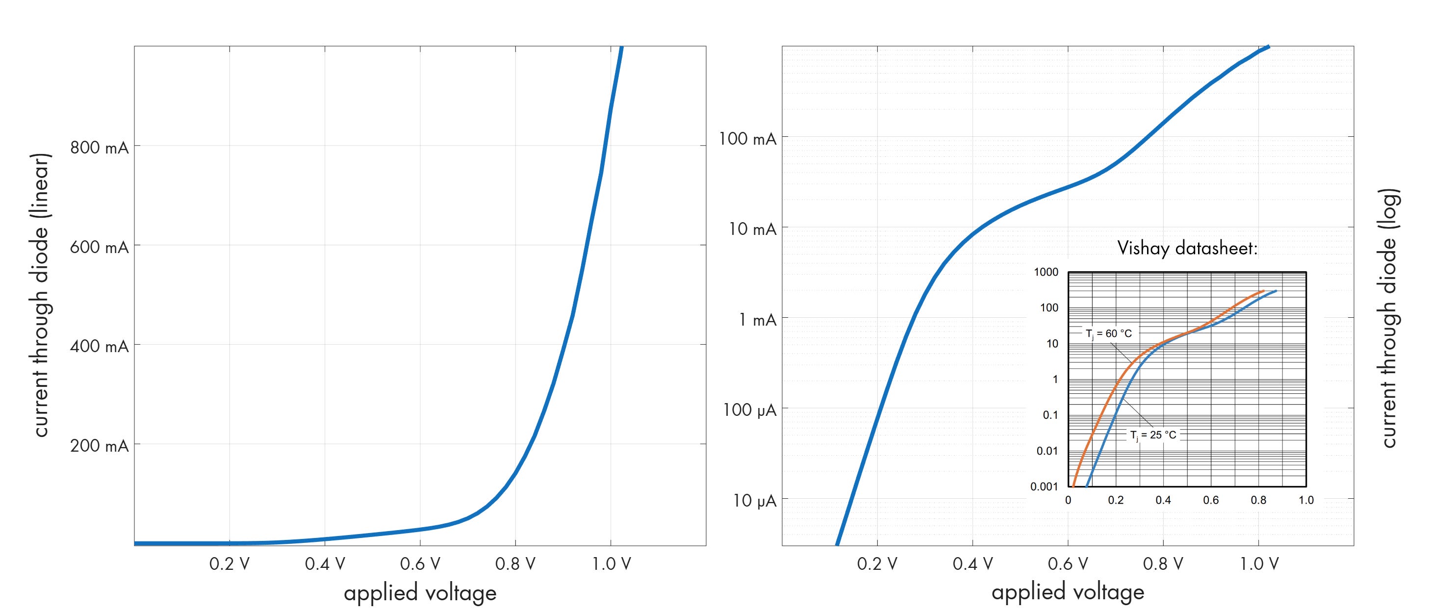
Some common diodes have unusual V-I curves. Here’s the capture for BAT46, a small Schottky diode. This is not an error! The inset shows the illustration from the Vishay datasheet:
The same toolkit also works for transistors. For example, here’s my plot of the admitted current in relation to the drain-source voltage for a small MOSFET, BS170:
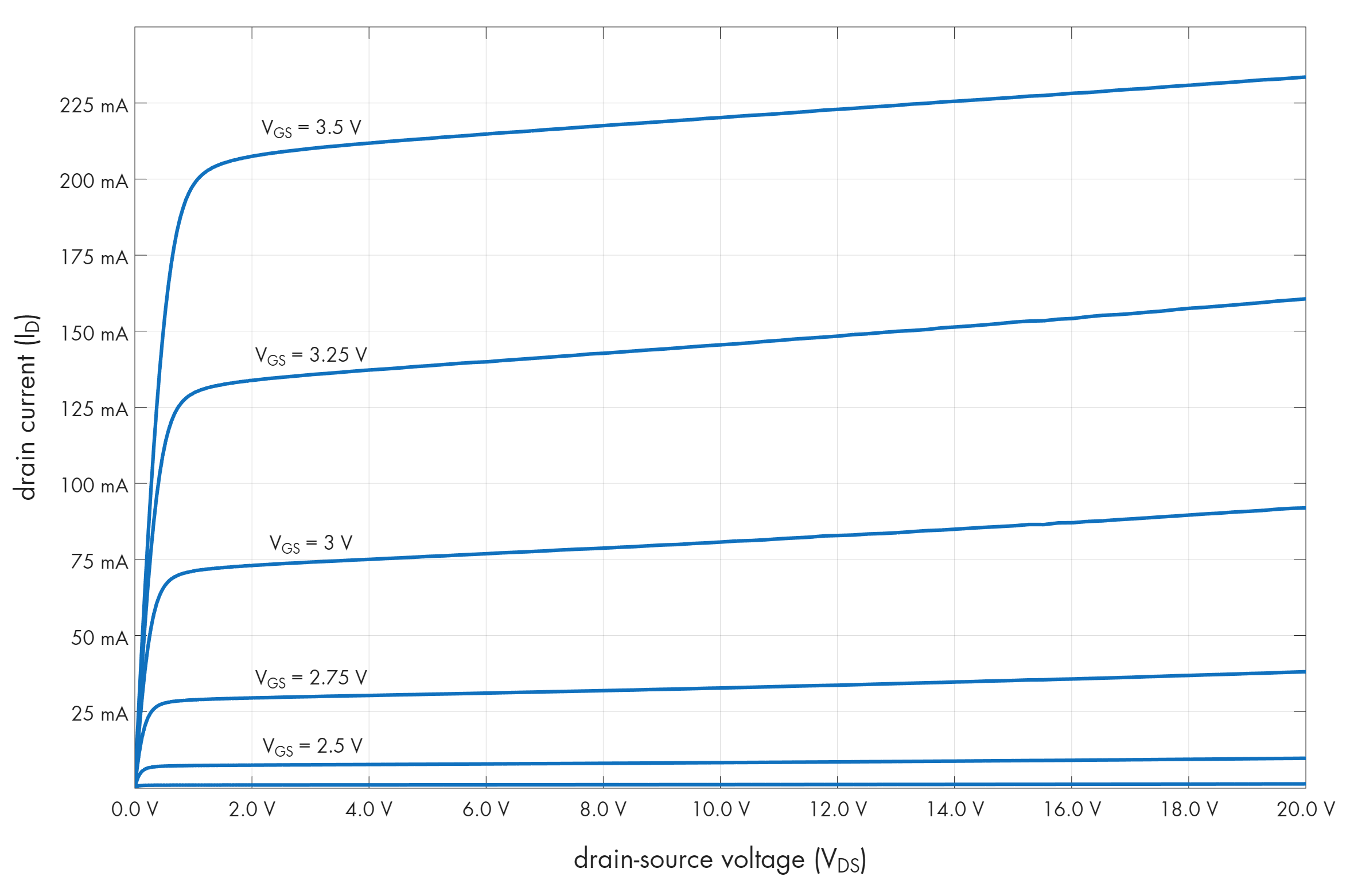
The plot shows that the transistor is more or less a constant-current device in the bulk of its usual operating range; the current limit is dialed in by the gate-source voltage (VGS) and changes less than 10% for VDS between 1 and 10 V.
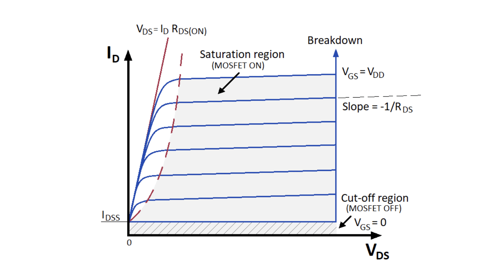
We can also show what happens on the tail end of that curve. The spec for the transistor gives its breakdown voltage as 60 V; in textbooks, this is usually shown as a sharp transition to vertical. For example, variants of the following diagram have made it into countless online articles and scientific papers:
Yet, the reality is more nuanced:
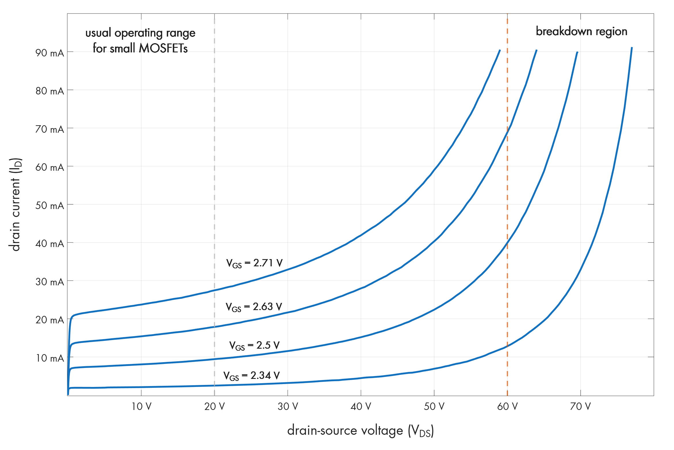
In a nutshell, you get a relatively sharp and spec-compliant breakdown only at very low gate voltages; in fact, the behavior is diode-like for VGS = 0 V (not shown above). But if you’re supplying a more practically useful VGS, the build-up to the danger zone is more gradual and you’ll be in trouble well ahead of 60 V.
As a side note, that last plot required a bit of ingenuity: my source measure unit has a limit of 20 V. To gain extra range, I added a traditional, floating power supply in series with the SMU and then stitched the captures for several voltage spans. This solved one problem but created another: even with the SMU idling, there would be substantial drain-source voltage applied to the device under test, and for some values of VGS, it could be enough to heat up or even destroy the transistor.
To address the issue, I moved from a fixed VGS signal to 1 millisecond pulses delivered by a signal generator at a 1% duty cycle. I also modified the data logging code to sample the current continuously over the period of about 2.5 seconds, average the best results, and then move to the next voltage set point. Source code for this variant can be found here.
By the way, you might find interesting discrepancies with manufacturer’s specs! On the left, you can see the VDS-ID diagram taken from the Microchip datasheet for 2N7000, a popular low-power MOSFET. In the middle, you can see my data, drawn to the same scale:
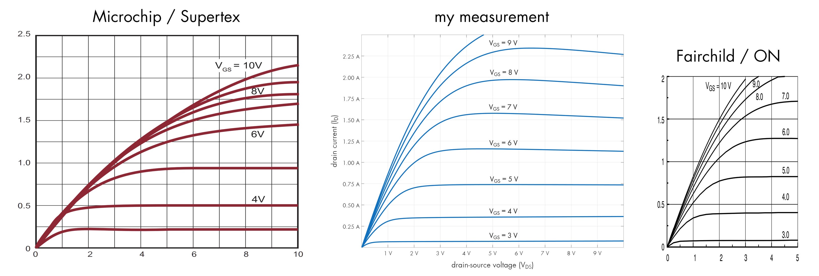
Although some batch-to-batch differences are to be expected, especially on the vertical axis, the two plots don’t line up the slightest. The scale-corrected diagram taken from the Fairchild / ON Semiconductor spec for the same transistor (right) aligns with my results nearly perfectly.
And yep, to preempt the inevitable comment: we used to have even more specialized devices, called "curve tracers", that were designed specifically for making V-I plots. They're more or less extinct now because SMUs can do the same job (including models that go to 200 V, 1,000 V, or even 3,000 V).
Great work! I am waiting for your new book. I noticed that text book curves don’t agree with oscilloscopes for power supplies. Seeing the truth is what I desire even if, the text book curves are ideal.